
Problems, steps and loads
A model is the structure; a problem is what happens to it. A problem is a sequence of steps, applied in order; each step has its loads and the results it should keep. One model can have several problems, say the serviceability and the ultimate checks, each solved and read on its own.
problem = model.add_problem(Problem(name="gravity_then_wind"))
dead = problem.add_step(StaticStep(name="dead_load"))dead.add_gravity_field(g=9810)                                   # self-weight, down z
wind = problem.add_step(StaticStep(name="wind"))                 # starts where dead_load left offwind.add_uniform_forcefield(nodes=left_eave, x=10_000)
for step in (dead, wind):    step.add_field_outputs([DisplacementFieldResults(), ReactionFieldResults()])
Kinds of analysis
Section titled “Kinds of analysis”| Step | Answers |
|---|---|
StaticStep |
Equilibrium under loads applied slowly: deflections, forces, stresses. nlgeom=True for large displacements; contact, one-way members and plasticity make it nonlinear by themselves. |
ModalAnalysis(modes) |
Natural frequencies and mode shapes, in the state the step before left. |
BucklingAnalysis(modes) |
The factors on the loads of the steps before at which the structure buckles. |
HeatTransferStep |
Temperatures: steady state, or in time, as under a fire curve. |
DynamicStep |
Loads that vary in time, with the model’s inertia. |
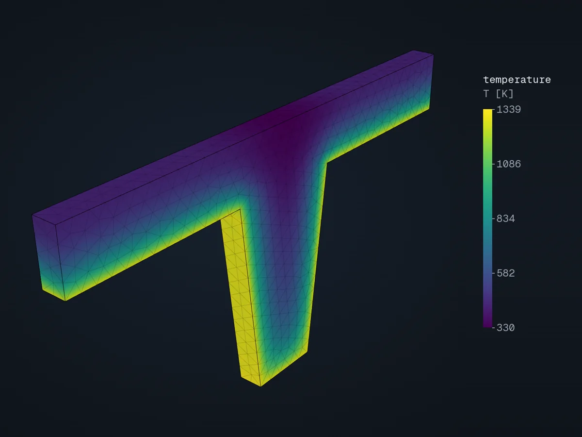
A heat transfer step: a ribbed slab after two hours of ISO 834 fire on its underside.
| Load | On | Method |
|---|---|---|
| Forces and moments at nodes | nodes | step.add_uniform_forcefield(nodes, x=, y=, z=, xx=, yy=, zz=) |
| Load per length | beams, bars | step.add_uniform_line_load(elements, z=-q) |
| Load per area (pressure) | element faces | step.add_surface_field(faces, z=-p) |
| Self-weight | elements | step.add_gravity_field(g=9810) |
| Prescribed displacements | nodes | step.add_uniform_displacement_field(nodes, ...) |
| Temperatures | nodes | step.add_temperature_field(...) |
A force field puts its full value on every node it is given: to spread a total force F over n nodes, give F / n, or use a line or surface load, which distribute it for you. Loads are in the global axes.
Load cases and combinations
Section titled “Load cases and combinations”Give each load a load_case, then add a combination to a step: the step is solved for the factored loads.
dead.add_gravity_field(g=9810, load_case="G")dead.add_uniform_line_load(rafter, z=-q_snow, load_case="Q")dead.add_combination(LoadFieldsCombination({"G": 1.35, "Q": 1.5}))The common design codes are ready-made: LoadFieldsCombination.ec_uls_persistent() (EN 1990, 6.10),
.ec_sls_characteristic(), .ec_uls_accidental() and the rest, and ASCE 7’s (.asce7_lrfd_basic(), …).
Running
Section titled “Running”problem.analyse_and_extract(path="output")One call has the input written, runs the solver on your machine, follows the solve and reads the results. A long
solve can be watched from a terminal (xfea status output -f) or by your AI assistant; every solve leaves a run
record and a one-page report. See Checking a model.
In the examples
Section titled “In the examples”- A static step, materially non-linear, modal and buckling.
- Line loads and tributary areas.
- Thermal and fire.
- Coulomb friction: two steps, a press then a push.
Analysis and Loads go through them step by step; the API reference has steps and loads.
© 2026 Francesco Ranaudo · Text and pictures CC BY 4.0 · Code Elastic License 2.0 · how to reuse them