
2D steady-state thermal analysis of a shell plate
A rectangular steel plate is subjected to a fixed temperature on its two short edges (hot side at x=0, cold side at x=L). The 1D steady-state heat equation yields a linear temperature distribution:
T(x) = T_hot + (T_cold - T_hot) × x / LThis linear profile is easy to verify in the FEA results.
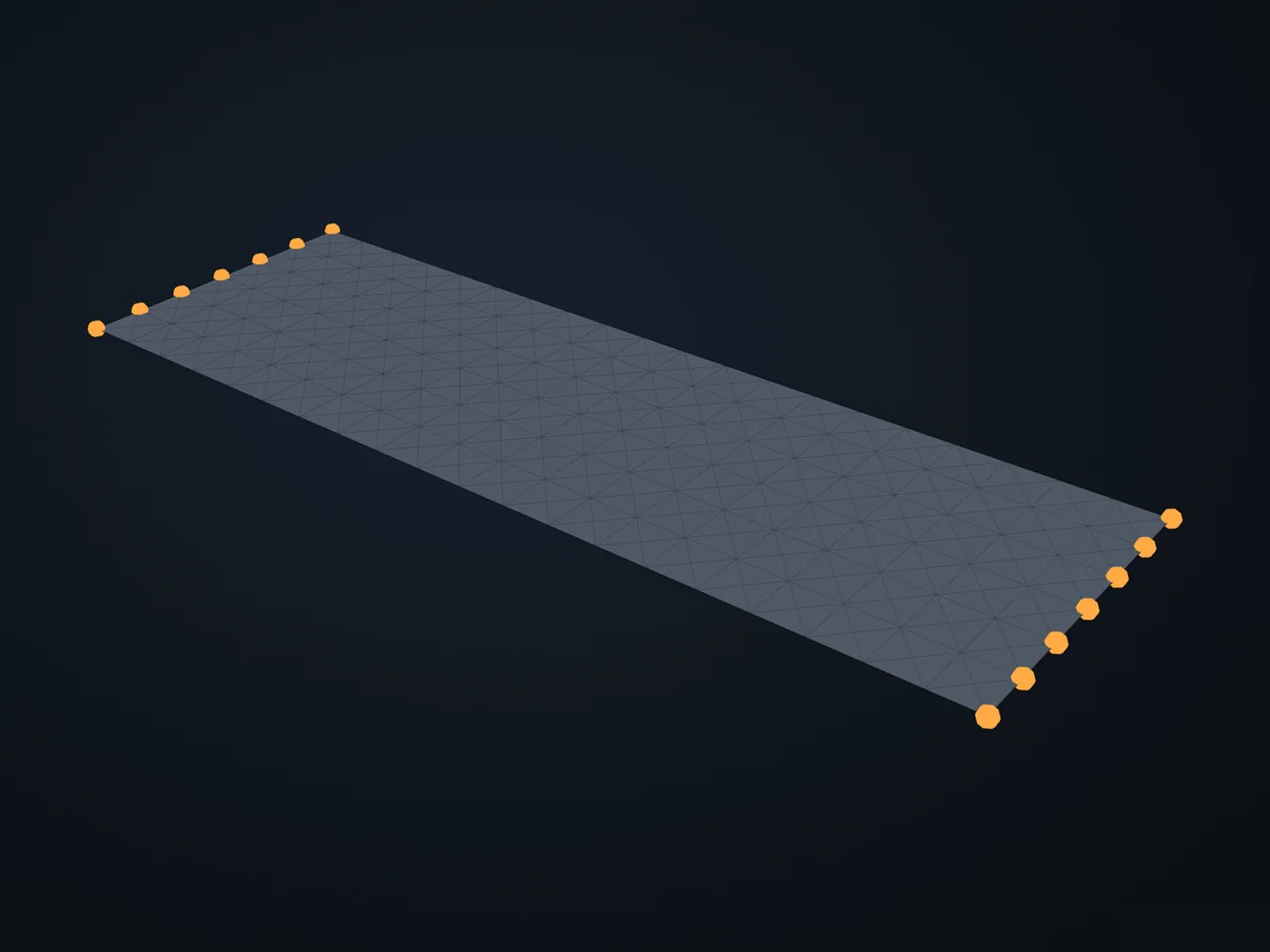
The model before it is solved: its parts, supports (red) and loads (blue).
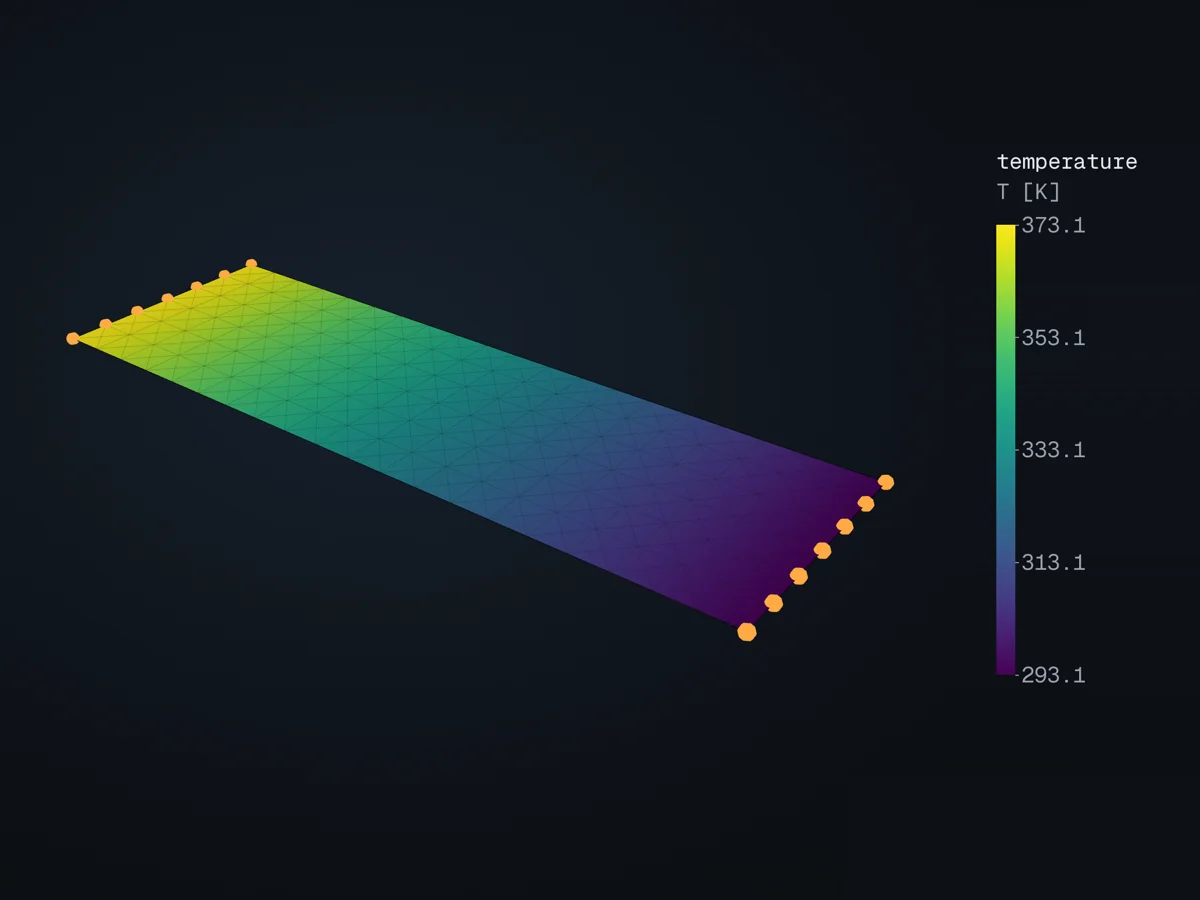
The model, coloured by temperature (T [K]), in xfea’s 3D viewer.
Open in 3D turn it, cut it, pick any field: in xfea's viewer, in your browser
The script
Section titled “The script”examples/scripts/02_core_concepts/thermal_analysis/thermal_plate.py. Run it from the repository with uv run python examples/scripts/02_core_concepts/thermal_analysis/thermal_plate.py, or, with xfea-examples installed, xfea-examples run 02_core_concepts/thermal_analysis/thermal_plate.py.
import matplotlib.pyplot as pltimport numpy as npfrom xfea.geometry import Mesh
from xfea.meshing import MeshingSettingsfrom xfea.model import Modelfrom xfea.model import Partfrom xfea.model import ShellSectionfrom xfea.model import ThermalElasticIsotropicfrom xfea.problem import HeatTransferStepfrom xfea.problem import Problemfrom xfea.results import TemperatureFieldResults
from xfea_examples import out_dirfrom xfea_examples import show_viewer
# Material — steel with thermal properties (SI-mm)k_steel = 45.0        # [mW/(mm*K)]     thermal conductivity (= 45 W/(m*K))c_steel = 500.0e6     # [mm^2/(s^2*K)]  specific heat (= 500 J/(kg*K) * 1e6)E_steel = 210_000     # [MPa]           Young's modulus (structural, unused here)v_steel = 0.3         # [-]             Poisson's ratiorho_steel = 7.85e-9   # [t/mm^3]        mass density
mat = ThermalElasticIsotropic(    k=k_steel,    c=c_steel,    E=E_steel,    v=v_steel,    density=rho_steel,)
# Geometry and sectionlength = 3000      # [mm] plate lengthwidth = 1000       # [mm] plate widththickness = 10     # [mm] shell thicknessnx = 20  # divisions along lengthny = 6   # divisions along widthmesh_min = 100     # [mm] target min element sizemesh_max = 200     # [mm] target max element size
sec = ShellSection(t=thickness, material=mat, int_points=3)
# Modelmodel = Model(name="thermal_plate")with model:    part = model.add_part(Part(name="plate"))    part.base_geometry = Mesh.from_meshgrid(length, nx, width, ny)    part.mesh(settings=MeshingSettings(min=mesh_min, max=mesh_max), section=sec)

# Temperature boundary conditionsT_hot = 373.15   # [K] prescribed hot-edge temperature (100 °C)T_cold = 293.15  # [K] prescribed cold-edge temperature (20 °C)
hot_nodes = part.nodes.subgroup(lambda n: n.x == 0)cold_nodes = part.nodes.subgroup(lambda n: n.x == length)
# Initial uniform temperature (the solver's heat-transfer analysis needs one)model.add_uniform_thermal_ics_field(T0=T_cold, nodes=part.nodes)model.add_thermal_bc(nodes=hot_nodes, temperature=T_hot)model.add_thermal_bc(nodes=cold_nodes, temperature=T_cold)
# Problem — single-increment steady-stateproblem = model.add_problem(Problem(name="thermal_plate"))step = problem.add_step(    HeatTransferStep(        name="steady_state",        steady_state=True,    ))
temp = TemperatureFieldResults()step.add_field_outputs([temp])
# Analysisproblem.analyse_and_extract(path=out_dir(model.name), verbose=True)
# Verification — boundary temperatures recoveredmin_temp = temp.get_min_result("T")max_temp = temp.get_max_result("T")
print("Steady-state thermal analysis")print(f"- Prescribed T_hot (x=0):  {T_hot:.2f} K  ({T_hot - 273.15:.1f} °C)")print(f"- Prescribed T_cold (x=L): {T_cold:.2f} K  ({T_cold - 273.15:.1f} °C)")print(f"- Min FEA temperature:     {min_temp.T}")print(f"- Max FEA temperature:     {max_temp.T}")print(f"  (Expected: min ≈ {T_cold:.1f} K, max ≈ {T_hot:.1f} K)")
# Verification plot — compare FEA temperatures against analytical solutionall_results = temp.resultsxs = np.array([r.location._x for r in all_results])ys = np.array([r.location._y for r in all_results])temps = np.array([float(r.T) for r in all_results])
T_analytical = T_hot + (T_cold - T_hot) * xs / length
fig, axes = plt.subplots(1, 2, figsize=(14, 5))
# Left: 2D temperature contourtri = axes[0].tricontourf(xs, ys, temps, levels=32, cmap="coolwarm")fig.colorbar(tri, ax=axes[0], label="Temperature [K]")axes[0].set_xlabel("x [mm]")axes[0].set_ylabel("y [mm]")axes[0].set_title("FEA Temperature Field")axes[0].set_aspect("equal")
# Right: T(x) profile vs analytical solutionaxes[1].scatter(xs, temps, s=8, alpha=0.5, label="FEA nodes")x_line = np.linspace(0, length, 200)axes[1].plot(    x_line,    T_hot + (T_cold - T_hot) * x_line / length,    "r-",    linewidth=2,    label="Analytical: T(x)",)axes[1].set_xlabel("x [mm]")axes[1].set_ylabel("Temperature [K]")axes[1].set_title("Temperature Profile Along Plate Length")axes[1].legend()axes[1].grid(True, alpha=0.3)
max_error = np.max(np.abs(temps - T_analytical))fig.suptitle(    f"Thermal Plate Verification — Max Error: {max_error:.2f} K",    fontsize=13,    fontweight="bold",)fig.tight_layout()
plot_path = out_dir(model.name) + "/thermal_plate_verification.png"fig.savefig(plot_path, dpi=150)print(f"\nVerification plot saved to: {plot_path}")plt.close(fig)
# Viewershow_viewer(model, results={temp: "T"}, units="K")© 2026 Francesco Ranaudo · Text and pictures CC BY 4.0 · Code Elastic License 2.0 · how to reuse them