
3D steady-state thermal analysis of a solid brick plate
A rectangular steel block is subjected to a fixed temperature on its two short faces (hot side at x=0, cold side at x=L). The 1D steady-state heat equation yields a linear temperature distribution:
T(x) = T_hot + (T_cold - T_hot) × x / LThis is the 3D solid-element counterpart of the shell-element thermal_plate
example. The analytical solution is identical; only the element type and
section differ.
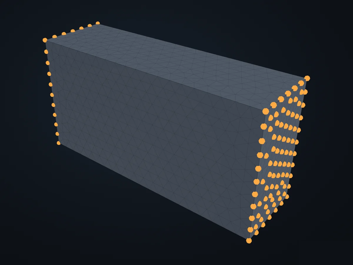
The model before it is solved: its parts, supports (red) and loads (blue).
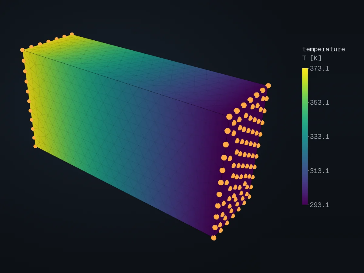
The model, coloured by temperature (T [K]), in xfea’s 3D viewer.
Open in 3D turn it, cut it, pick any field: in xfea's viewer, in your browser
The script
Section titled “The script”examples/scripts/02_core_concepts/thermal_analysis/thermal_solid.py. Run it from the repository with uv run python examples/scripts/02_core_concepts/thermal_analysis/thermal_solid.py, or, with xfea-examples installed, xfea-examples run 02_core_concepts/thermal_analysis/thermal_solid.py.
import os
import matplotlib.pyplot as pltimport numpy as np
from xfea.meshing import MeshingSettingsfrom xfea.model import Modelfrom xfea.model import Partfrom xfea.model import SolidSectionfrom xfea.model import ThermalElasticIsotropicfrom xfea.problem import HeatTransferStepfrom xfea.problem import Problemfrom xfea.results import TemperatureFieldResults
from xfea_examples import out_dirfrom xfea_examples.step import box_stepfrom xfea_examples import show_viewerfrom xfea_examples.models import _nodes_at_extremefrom xfea_tools import CuttingPlane, plot_cross_section
# Material — steel with thermal properties (SI-mm)k_steel = 45.0          # [mW/(mm*K)]     thermal conductivity (= 45 W/(m*K))c_steel = 500.0e6       # [mm^2/(s^2*K)]  specific heat (= 500 J/(kg*K) * 1e6)E_steel = 210_000       # [MPa]           Young's modulus (structural, unused here)v_steel = 0.3           # [-]             Poisson's ratiorho_steel = 7.85e-9     # [t/mm^3]        mass density
mat = ThermalElasticIsotropic(    k=k_steel,    c=c_steel,    E=E_steel,    v=v_steel,    density=rho_steel,)
# Geometry and sectionlength = 1000     # [mm] block lengthwidth = 300       # [mm] block widththickness = 500   # [mm] block thicknessmesh_min = 10     # [mm] target min element sizemesh_max = 50     # [mm] target max element size
sec = SolidSection(material=mat)
# Model# The plate's geometry, x in [0, length], y in [0, width], z in [0, thickness], as a STEP file next to the resultsstep_path = box_step(os.path.join(out_dir("thermal_solid"), "thermal_plate_solid.stp"), length, width, thickness)
model = Model(name="thermal_solid")part = model.add_part(Part(name="solid"))part.base_geometry = step_pathpart.mesh(settings=MeshingSettings(min=mesh_min, max=mesh_max), section=sec)
# Temperature boundary conditionsT_hot = 373.15   # [K] prescribed hot-face temperature (100 °C)T_cold = 293.15  # [K] prescribed cold-face temperature (20 °C)
hot_nodes = _nodes_at_extreme(part.nodes, axis="x", mode="min")cold_nodes = _nodes_at_extreme(part.nodes, axis="x", mode="max")
# Initial uniform temperature (the solver's heat-transfer analysis needs one)model.add_uniform_thermal_ics_field(T0=T_cold, nodes=part.nodes)model.add_thermal_bc(nodes=hot_nodes, temperature=T_hot)model.add_thermal_bc(nodes=cold_nodes, temperature=T_cold)
# Problem — single-increment steady-stateproblem = model.add_problem(Problem(name="thermal_solid"))step = problem.add_step(    HeatTransferStep(        name="steady_state",        steady_state=True,    ))
temp = TemperatureFieldResults()step.add_field_outputs([temp])
# Analysisproblem.analyse_and_extract(path=out_dir(model.name), verbose=True)
# Verification — boundary temperatures recoveredmin_temp = temp.get_min_result("T")max_temp = temp.get_max_result("T")
print("Steady-state thermal analysis — 3D solid elements")print(f"- Prescribed T_hot (x=0):  {T_hot:.2f} K  ({T_hot - 273.15:.1f} °C)")print(f"- Prescribed T_cold (x=L): {T_cold:.2f} K  ({T_cold - 273.15:.1f} °C)")print(f"- Min FEA temperature:     {min_temp.T}")print(f"- Max FEA temperature:     {max_temp.T}")print(f"  (Expected: min ≈ {T_cold:.1f} K, max ≈ {T_hot:.1f} K)")
# Verification plot — compare FEA temperatures against analytical solutionall_results = temp.resultsxs = np.array([r.location._x for r in all_results])ys = np.array([r.location._y for r in all_results])temps = np.array([float(r.T) for r in all_results])
T_analytical = T_hot + (T_cold - T_hot) * xs / length
fig, axes = plt.subplots(1, 2, figsize=(14, 5))
# Left: 2D temperature contour (XY projection — all nodes across thickness)tri = axes[0].tricontourf(xs, ys, temps, levels=32, cmap="coolwarm")fig.colorbar(tri, ax=axes[0], label="Temperature [K]")axes[0].set_xlabel("x [mm]")axes[0].set_ylabel("y [mm]")axes[0].set_title("FEA Temperature Field (XY projection)")axes[0].set_aspect("equal")
# Right: T(x) profile vs analytical solutionaxes[1].scatter(xs, temps, s=8, alpha=0.5, label="FEA nodes")x_line = np.linspace(0, length, 200)axes[1].plot(    x_line,    T_hot + (T_cold - T_hot) * x_line / length,    "r-",    linewidth=2,    label="Analytical: T(x)",)axes[1].set_xlabel("x [mm]")axes[1].set_ylabel("Temperature [K]")axes[1].set_title("Temperature Profile Along Plate Length")axes[1].legend()axes[1].grid(True, alpha=0.3)
max_error = np.max(np.abs(temps - T_analytical))fig.suptitle(    f"Thermal Solid Verification — Max Error: {max_error:.2f} K",    fontsize=13,    fontweight="bold",)fig.tight_layout()
plot_path = out_dir(model.name) + "/thermal_solid_verification.png"fig.savefig(plot_path, dpi=150)print(f"\nVerification plot saved to: {plot_path}")plt.close(fig)
# Cross-section cuts using xfea_tools
# Cut at mid-length (x = length / 2): expect a uniform T ~ 333.15 K across the sectionplane_mid = CuttingPlane(axis="x", value=length / 2, tolerance=50)fig, ax = plot_cross_section(    temp, "T", plane_mid,    colorbar_label="Temperature [K]",    title=f"Cross-section at x={length / 2:.0f} mm",)cs_path = out_dir(model.name) + "/cross_section_midplane.png"fig.savefig(cs_path, dpi=150)print(f"Cross-section plot saved to: {cs_path}")plt.close(fig)
# Cut along the mid spine (y)plane_quarter = CuttingPlane(axis="y", value=width / 2, tolerance=50)fig, ax = plot_cross_section(    temp, "T", plane_quarter,    colorbar_label="Temperature [K]",)cs_path2 = out_dir(model.name) + "/cross_section_mid.png"fig.savefig(cs_path2, dpi=150)print(f"Cross-section plot saved to: {cs_path2}")plt.close(fig)
# Viewer# Opens the viewer when asked to (XFEA_EXAMPLES_SHOW_VIEWER=1); in an unattended run it would wait for ever.show_viewer(model, results={temp: "T"}, units="K")© 2026 Francesco Ranaudo · Text and pictures CC BY 4.0 · Code Elastic License 2.0 · how to reuse them