
Iterative filtering of a solid thermal model
Starting from the thermal_solid setup (3D steady-state heat transfer on a
steel block), this script demonstrates the filter_model tool from
xfea_tools:
- Run the initial thermal analysis.
- Remove all elements where T > 350 K (the “hot zone”).
- Visualise what was removed.
- Re-analyse the filtered model with new boundary conditions.
This pattern — analyse → filter → re-analyse — is the basis for iterative workflows such as progressive damage modelling, adaptive mesh refinement, or topology-optimisation-style loops.
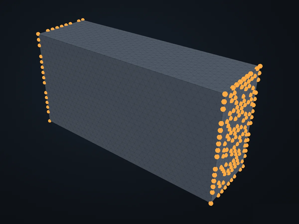
The model before it is solved: its parts, supports (red) and loads (blue).
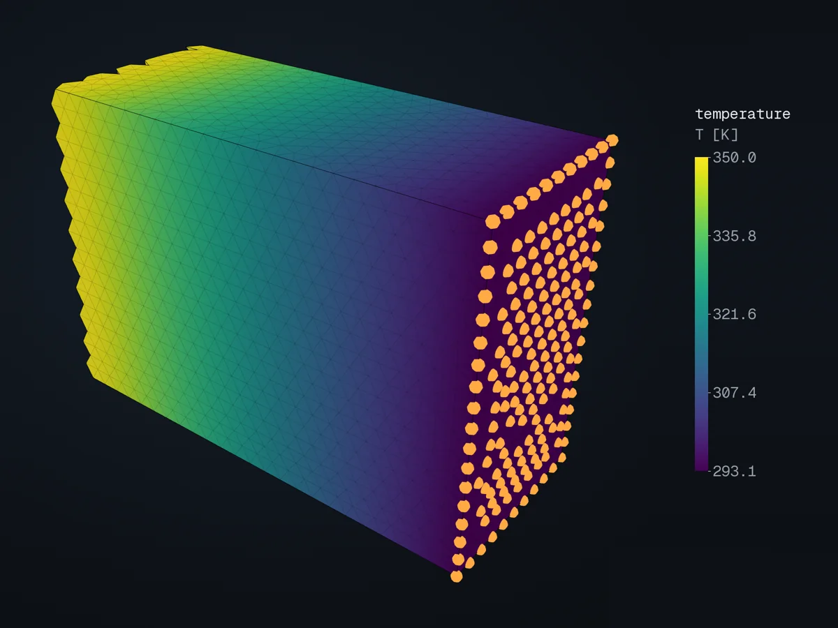
The model, coloured by temperature (T [K]), in xfea’s 3D viewer.
Open in 3D turn it, cut it, pick any field: in xfea's viewer, in your browser
The script
Section titled “The script”examples/scripts/02_core_concepts/thermal_analysis/thermal_solid_filter.py. Run it from the repository with uv run python examples/scripts/02_core_concepts/thermal_analysis/thermal_solid_filter.py, or, with xfea-examples installed, xfea-examples run 02_core_concepts/thermal_analysis/thermal_solid_filter.py.
import os
import matplotlib.pyplot as pltimport numpy as np
from xfea.meshing import MeshingSettingsfrom xfea.model import Modelfrom xfea.model import Partfrom xfea.model import SolidSectionfrom xfea.model import ThermalElasticIsotropicfrom xfea.problem import HeatTransferStepfrom xfea.problem import Problemfrom xfea.results import TemperatureFieldResults
from xfea_examples import out_dirfrom xfea_examples.step import box_stepfrom xfea_examples import show_viewerfrom xfea_examples.models import _nodes_at_extremefrom xfea_tools import CuttingPlanefrom xfea_tools import filter_modelfrom xfea_tools import plot_cross_section
# Material — steel with thermal properties (SI-mm)k_steel = 45.0        # [mW/(mm*K)]     thermal conductivity (= 45 W/(m*K))c_steel = 500.0e6     # [mm^2/(s^2*K)]  specific heat (= 500 J/(kg*K) * 1e6)E_steel = 210_000     # [MPa]           Young's modulus (structural, unused here)v_steel = 0.3         # [-]             Poisson's ratiorho_steel = 7.85e-9   # [t/mm^3]        mass density
mat = ThermalElasticIsotropic(    k=k_steel,    c=c_steel,    E=E_steel,    v=v_steel,    density=rho_steel,)
# Geometrylength = 1000       # [mm] block lengthwidth = 300         # [mm] block widththickness = 500     # [mm] block thicknessmesh_min = 5        # [mm] target min element sizemesh_max = 30       # [mm] target max element sizesec = SolidSection(material=mat)
# The plate's geometry, as a STEP file next to the resultsstep_path = box_step(os.path.join(out_dir("thermal_solid_filter"), "thermal_plate_solid.stp"), length, width, thickness)
# Original modelmodel = Model(name="thermal_solid_filter")with model:    part = model.add_part(Part(name="solid"))    part.base_geometry = step_path    part.mesh(settings=MeshingSettings(min=mesh_min, max=mesh_max), section=sec)
T_hot = 373.15   # [K] prescribed hot-face temperature (100 °C)T_cold = 293.15  # [K] prescribed cold-face temperature (20 °C)
hot_nodes = _nodes_at_extreme(part.nodes, axis="x", mode="min")cold_nodes = _nodes_at_extreme(part.nodes, axis="x", mode="max")
model.add_uniform_thermal_ics_field(T0=T_cold, nodes=part.nodes)model.add_thermal_bc(nodes=hot_nodes, temperature=T_hot)model.add_thermal_bc(nodes=cold_nodes, temperature=T_cold)
problem = model.add_problem(Problem(name="thermal_solid_filter"))step = problem.add_step(    HeatTransferStep(name="steady_state", steady_state=True))
temp = TemperatureFieldResults()step.add_field_outputs([temp])
# Step 1 — Analyse the original modelprint("=" * 60)print("Step 1: Analysing original model")print("=" * 60)problem.analyse_and_extract(path=out_dir(model.name), verbose=True)
n_orig = len(part.elements or [])print(f"\nOriginal model: {n_orig} elements")
# Step 2 — Filter: remove elements where T > 350 KT_THRESHOLD = 350.0  # [K] filter threshold
print(f"\n{'=' * 60}")print(f"Step 2: Filtering — removing elements where T > {T_THRESHOLD} K")print("=" * 60)
filtered = filter_model(    model, temp, "T",    condition=lambda T: T > T_THRESHOLD,    mode="remove",    cleanup_orphans=True,    smooth=5,)
filtered_part = list(filtered.parts)[0]n_filtered = len(filtered_part.elements or [])n_removed = n_orig - n_filteredprint(f"Filtered model: {n_filtered} elements ({n_removed} removed, {n_removed / n_orig:.0%} of total)")
# Step 3 — Re-analyse the filtered model with different BCsprint(f"\n{'=' * 60}")print("Step 3: Re-analysing filtered model (clean — no old results)")print("=" * 60)
filtered.name = "thermal_solid_filtered"
# The cut surface is held at the threshold temperature, the cold face as before: a different# temperature profile from the original, showing that the filtered model is truly independent.# The cut is ragged (it follows the removed elements, then smoothed), so it is found as the boundary# nodes that were not on the block's six faces, not as the nodes at the smallest x (one node, here).def _on_block_face(n, tol=1e-6):    x, y, z = n.xyz    return (abs(x) < tol or abs(x - length) < tol or abs(y) < tol or abs(y - width) < tol            or abs(z) < tol or abs(z - thickness) < tol)

cut_face = filtered_part.find_boundary_nodes().subgroup(lambda n: not _on_block_face(n))filtered_max_x = _nodes_at_extreme(filtered_part.nodes, axis="x", mode="max")print(f"Cut surface: {len(cut_face)} nodes, held at {T_THRESHOLD} K")
filtered.add_uniform_thermal_ics_field(T0=T_cold, nodes=filtered_part.nodes)filtered.add_thermal_bc(nodes=cut_face, temperature=T_THRESHOLD)  # cut surface: threshold Tfiltered.add_thermal_bc(nodes=filtered_max_x, temperature=T_cold)       # cold face: same as before
problem2 = filtered.add_problem(Problem(name="thermal_solid_filtered"))step2 = problem2.add_step(    HeatTransferStep(name="steady_state", steady_state=True))temp2 = TemperatureFieldResults()step2.add_field_outputs([temp2])
problem2.analyse_and_extract(path=out_dir(filtered.name), verbose=True)
# Step 4 — Comparison plotsprint(f"\n{'=' * 60}")print("Step 4: Visualisation")print("=" * 60)
fig, axes = plt.subplots(1, 3, figsize=(20, 5))
# Collect original resultsr_orig = temp.resultsxs_o = np.array([r.location._x for r in r_orig])ys_o = np.array([r.location._y for r in r_orig])ts_o = np.array([float(r.T) for r in r_orig])
# --- Panel 1: Original temperature field ---tri0 = axes[0].tricontourf(xs_o, ys_o, ts_o, levels=32, cmap="coolwarm")fig.colorbar(tri0, ax=axes[0], label="Temperature [K]")axes[0].axvline(x=min(r.location._x for r in temp2.results), color="k",                linestyle="--", linewidth=1.5, label="cut boundary")axes[0].legend(loc="lower left", fontsize=8)axes[0].set_xlabel("x [mm]")axes[0].set_ylabel("y [mm]")axes[0].set_title(f"1. Original ({n_orig} elements)")axes[0].set_aspect("equal")
# --- Panel 2: Which elements were removed (scatter) ---# Colour the original nodes by whether they survived filteringfiltered_node_xs = set()for n in filtered_part.nodes:    filtered_node_xs.add(round(n._x, 2))
survived = np.array([round(r.location._x, 2) in filtered_node_xs for r in r_orig])
axes[1].scatter(xs_o[~survived], ys_o[~survived], c="red", s=3, alpha=0.6, label="removed")axes[1].scatter(xs_o[survived], ys_o[survived], c="steelblue", s=3, alpha=0.6, label="kept")axes[1].legend(fontsize=9)axes[1].set_xlabel("x [mm]")axes[1].set_ylabel("y [mm]")axes[1].set_title(f"2. Filter: T > {T_THRESHOLD} K → {n_removed} removed")axes[1].set_aspect("equal")
# --- Panel 3: Filtered model re-analysed ---r_filt = temp2.resultsxs_f = np.array([r.location._x for r in r_filt])ys_f = np.array([r.location._y for r in r_filt])ts_f = np.array([float(r.T) for r in r_filt])tri1 = axes[2].tricontourf(xs_f, ys_f, ts_f, levels=32, cmap="coolwarm")fig.colorbar(tri1, ax=axes[2], label="Temperature [K]")axes[2].set_xlabel("x [mm]")axes[2].set_ylabel("y [mm]")axes[2].set_title(f"3. Re-analysed ({n_filtered} elements)")axes[2].set_aspect("equal")
fig.suptitle(    f"Iterative Filtering: Remove Elements Where T > {T_THRESHOLD} K",    fontsize=13,    fontweight="bold",)fig.tight_layout()
plot_path = out_dir(model.name) + "/thermal_solid_filter_comparison.png"fig.savefig(plot_path, dpi=150)print(f"\nComparison plot saved to: {plot_path}")plt.close(fig)
# Cross-section of the filtered modelplane_mid = CuttingPlane(axis="y", value=width / 2, tolerance=50)fig_cs, ax_cs = plot_cross_section(    temp2, "T", plane_mid,    colorbar_label="Temperature [K]",    title=f"Filtered model — cross-section at y={width / 2:.0f} mm",)cs_path = out_dir(model.name) + "/thermal_solid_filter_cross_section.png"fig_cs.savefig(cs_path, dpi=150)print(f"Cross-section plot saved to: {cs_path}")plt.close(fig_cs)
# Viewershow_viewer(filtered, results={temp2: "T"}, units="K")© 2026 Francesco Ranaudo · Text and pictures CC BY 4.0 · Code Elastic License 2.0 · how to reuse them