
UniformLineLoadField for distributed loads on 1D members
Demonstrates step.add_uniform_line_load(...) and checks it against:
- The classical Euler-Bernoulli analytical solution for a simply- supported beam with a uniform UDL: δ_mid = 5 · q · L⁴ / (384 · E · I)
- The same load as lumped nodal forces computed by hand — both approaches should give the same FEA result, because the line load is lumped onto the nodes by the same trapezoidal rule.
Two FEA runs per mesh density:
(a) step.add_uniform_line_load(distribution=beams, magnitude=q, direction=[0, 0, -1]) — the line load.
(b) step.add_uniform_forcefield(...) with manually computed
q·dx/2 at end nodes and q·dx at interior nodes.
A matplotlib plot at the end shows: - mid deflection vs. mesh density for both approaches (they should be indistinguishable), - the analytical target line, - the % error shrinking with mesh refinement.
The beam cross-section is a plain rectangle, so the solver takes it exactly as defined (no section approximation enters the comparison).
Units: mm / N / MPa.
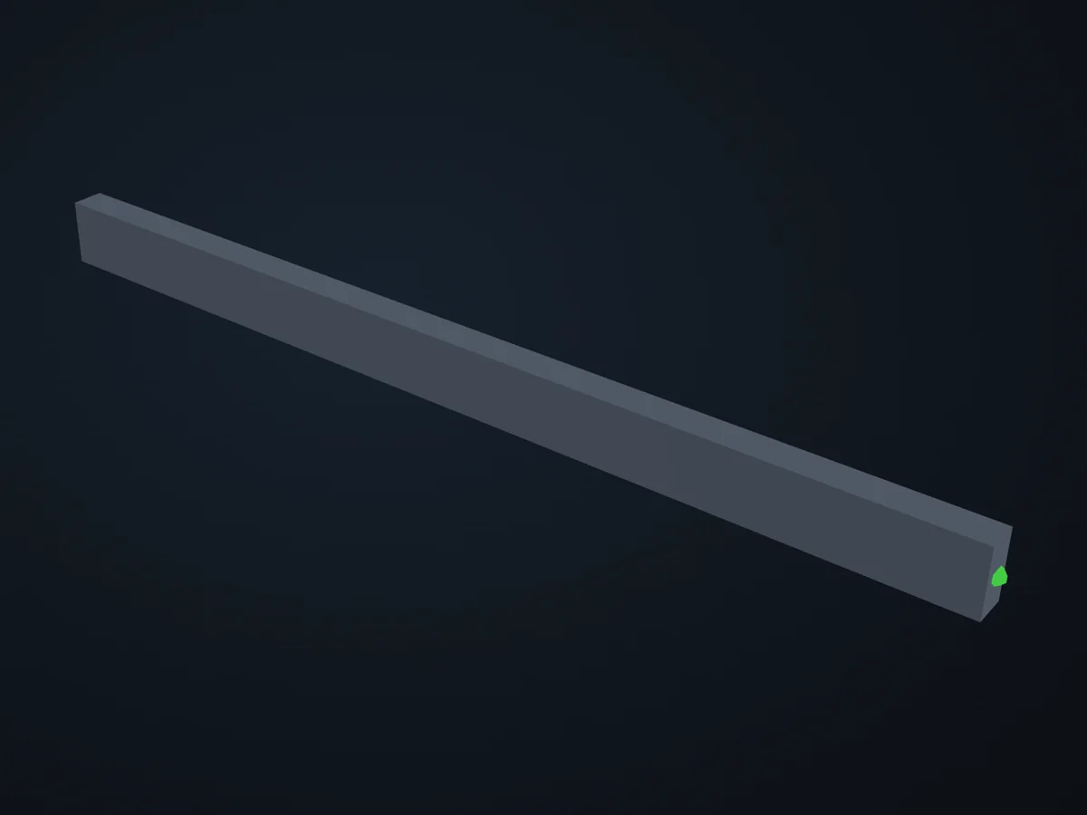
The model before it is solved: its parts, supports (red) and loads (blue).
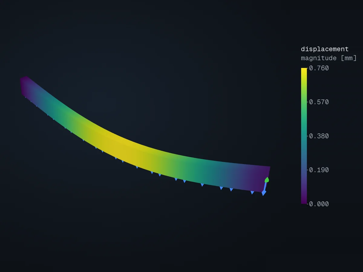
The deformed shape, coloured by displacement (magnitude [mm]), in xfea’s 3D viewer.
Open in 3D turn it, cut it, pick any field: in xfea's viewer, in your browser
The script
Section titled “The script”examples/scripts/02_core_concepts/loads_and_bcs/line_loads.py. Run it from the repository with uv run python examples/scripts/02_core_concepts/loads_and_bcs/line_loads.py, or, with xfea-examples installed, xfea-examples run 02_core_concepts/loads_and_bcs/line_loads.py.
from __future__ import annotations
import timefrom pathlib import Path
from xfea.model import (    BeamElement,    ElasticIsotropic,    Model,    Node,    Part,    RectangularSection,)from xfea.problem import (    Problem,    StaticStep,)from xfea.results import DisplacementFieldResults
from xfea_examples import out_dir

# Test case: simply-supported rectangular beam, 3 m span, UDL = 10 N/mmE = 210_000.0                 # [MPa]NU = 0.3DENSITY = 7.85e-9             # [t/mm³]
L_SPAN = 3_000.0              # [mm]Q = 10.0                      # [N/mm]  (10 kN/m downward UDL)
# 100 × 200 mm rectangular cross-sectionSEC_W = 100.0                 # [mm]  width along local 1 (orientation)SEC_H = 200.0                 # [mm]  height along local 2
# Analytical reference — Euler-Bernoulli simply-supported beam under UDL.# δ_mid = 5·q·L⁴ / (384·E·I)    R_end = q·L/2    M_mid = q·L²/8def analytical():    # Rectangular section bending about local 1 axis: I = w × h³ / 12.    # The RectangularSection stores that in ``Ixx`` (strong axis of    # the rectangle).  The beam bends under the -Z load about global Y,    # which with orientation=[0,1,0] maps to the beam's local 1 axis,    # so ``Ixx`` is the inertia we want.    I = SEC_W * SEC_H**3 / 12.0    delta_mid = -5.0 * Q * L_SPAN**4 / (384.0 * E * I)    return delta_mid, I

# Helpers — build the beam model, solve, and return the mid-span δz.

def _build_beam(n_elem: int, name: str):    """Return (model, nodes, beams) for a simply-supported rectangular beam    with ``n_elem`` linear beam elements along the span."""    steel = ElasticIsotropic(E=E, v=NU, density=DENSITY, name="S355")    sec = RectangularSection(w=SEC_W, h=SEC_H, material=steel, name="rect")    model = Model(name=name)    part = Part(name="beam")    model.add_part(part)    dx = L_SPAN / n_elem    nodes = [part.add_node(Node(xyz=[i * dx, 0.0, 0.0])) for i in range(n_elem + 1)]    beams = [        part.add_element(            BeamElement(                nodes=[nodes[i], nodes[i + 1]],                section=sec,                orientation=[0, 1, 0],   # strong-axis bending            )        )        for i in range(n_elem)    ]    model.add_pin_bc(nodes=[nodes[0]])        # pinned left end    model.add_rollerY_bc(nodes=[nodes[-1]])   # roller right end (y/z free)    return model, nodes, beams

def _solve_mid_deflection(problem, mid_node, step) -> float:    disp = DisplacementFieldResults()    step.add_field_outputs([disp])    out = out_dir(problem.name)    problem.analyse_and_extract(path=out, verbose=False)    return float(disp.get_result_at(mid_node, time=1.0).z)

def solve_with_line_load_api(n_elem: int) -> tuple[float, float]:    """Apply UDL as a :class:`UniformLineLoadField`."""    model, nodes, beams = _build_beam(        n_elem, name=f"ss_api_{n_elem:03d}"    )    problem = model.add_problem(Problem(name=f"ss_api_{n_elem:03d}"))    step = problem.add_step(StaticStep(name="udl"))    step.add_uniform_line_load(        distribution=beams, magnitude=Q, direction=[0, 0, -1]    )    t0 = time.perf_counter()    delta_mid = _solve_mid_deflection(problem, nodes[n_elem // 2], step)    wall = time.perf_counter() - t0    return delta_mid, wall

def solve_with_manual_nodal_loads(n_elem: int) -> tuple[float, float]:    """Apply UDL as nodal forces by the trapezoidal rule."""    model, nodes, _ = _build_beam(        n_elem, name=f"ss_manual_{n_elem:03d}"    )    problem = model.add_problem(Problem(name=f"ss_manual_{n_elem:03d}"))    step = problem.add_step(StaticStep(name="udl"))    dx = L_SPAN / n_elem    end_force = -Q * dx / 2    interior_force = -Q * dx    if len(nodes) >= 2:        step.add_uniform_forcefield(            nodes=[nodes[0], nodes[-1]], z=end_force        )    if len(nodes) > 2:        step.add_uniform_forcefield(nodes=nodes[1:-1], z=interior_force)    t0 = time.perf_counter()    delta_mid = _solve_mid_deflection(problem, nodes[n_elem // 2], step)    wall = time.perf_counter() - t0    return delta_mid, wall

# Benchmark runner + plotdef run_benchmark(mesh_sizes: list[int]):    delta_ref, I_y = analytical()    print("=" * 68)    print("Simply-supported 100×200 mm rectangular beam — UDL benchmark")    print("  L    = {:.0f} mm".format(L_SPAN))    print("  q    = {:.1f} N/mm   ({:.1f} kN/m)".format(Q, Q))    print("  E    = {:.0f} MPa   ν = {}".format(E, NU))    print("  I    = {:,.0f} mm⁴  (100 × 200³ / 12)".format(I_y))    print("  δ_mid (analytical) = 5qL⁴/(384·E·I) = {:+.6f} mm".format(delta_ref))    print("=" * 68)    print()    print(f"  {'n_elem':>6}  {'δ_api [mm]':>14}  {'err_api':>8}  "          f"{'δ_manual [mm]':>14}  {'err_man':>8}  {'t_api/t_man [s]':>16}")    rows = []    for n in mesh_sizes:        d_api, t_api = solve_with_line_load_api(n)        d_man, t_man = solve_with_manual_nodal_loads(n)        err_api = abs(d_api - delta_ref) / abs(delta_ref) * 100.0        err_man = abs(d_man - delta_ref) / abs(delta_ref) * 100.0        rows.append((n, d_api, err_api, d_man, err_man, t_api, t_man))        print(            f"  {n:>6d}  {d_api:>+14.6f}  {err_api:>7.3f}%  "            f"{d_man:>+14.6f}  {err_man:>7.3f}%  "            f"{t_api:>6.1f} / {t_man:<6.1f}"        )    return rows, delta_ref

def plot_convergence(rows, delta_ref):    import matplotlib.pyplot as plt
    ns = [r[0] for r in rows]    d_api = [r[1] for r in rows]    d_man = [r[3] for r in rows]    err_api = [r[2] for r in rows]    err_man = [r[4] for r in rows]
    fig, (ax1, ax2) = plt.subplots(1, 2, figsize=(12, 5))
    # Left: deflection vs mesh density    ax1.axhline(        delta_ref, color="black", lw=1.2, ls="--",        label=f"analytical  {delta_ref:+.4f} mm",    )    ax1.plot(ns, d_api, "o-", color="tab:blue", label="line-load API")    ax1.plot(ns, d_man, "s--", color="tab:orange", label="manual nodal loads",             markerfacecolor="none")    ax1.set_xscale("log", base=2)    ax1.set_xlabel("elements along span")    ax1.set_ylabel("mid-span δz (mm)")    ax1.set_title("FEA mid-span deflection")    ax1.grid(True, alpha=0.3)    ax1.legend(fontsize=9)
    # Right: %-error vs mesh density    ax2.plot(ns, err_api, "o-", color="tab:blue", label="line-load API")    ax2.plot(ns, err_man, "s--", color="tab:orange", label="manual nodal loads",             markerfacecolor="none")    ax2.set_xscale("log", base=2)    ax2.set_yscale("log")    ax2.set_xlabel("elements along span")    ax2.set_ylabel("|error| vs analytical (%)")    ax2.set_title("Convergence to analytical")    ax2.grid(True, which="both", alpha=0.3)    ax2.legend(fontsize=9)
    fig.suptitle(        "UniformLineLoadField benchmark — simply-supported 100×200 mm × 3 m, "        f"q = {Q:.0f} N/mm"    )    fig.tight_layout()    out = Path(out_dir("line_loads")) / "benchmark.png"    out.parent.mkdir(parents=True, exist_ok=True)    fig.savefig(out, dpi=150)    print(f"\n  convergence plot saved: {out}")    plt.show()

if __name__ == "__main__": rows, delta_ref = run_benchmark(mesh_sizes=[2, 4, 8, 16, 32]) plot_convergence(rows, delta_ref)© 2026 Francesco Ranaudo · Text and pictures CC BY 4.0 · Code Elastic License 2.0 · how to reuse them