
ForceField via step.add_tributary_area_load(...)
Demonstrates distributing a uniform area pressure onto a grid of
supporting beams without modelling the plate itself. The plate is
a pure geometric concept (a xfea.geometry.Polygon) — only the
ribs are in the FE mesh. The method produces concentrated nodal
forces at the ribs’ end-nodes with tributary areas integrated and
lumped on the fly.
Layout
Section titled “Layout”A 6 m × 4 m rectangular plate sitting on a grid of parallel beams:
─────────────────────────────────────────── y = 4.0│ ││ beam 3 ── rib spacing = 1 m │ ← y = 3.0│ ││ beam 2 │ ← y = 2.0│ ││ beam 1 │ ← y = 1.0│ ││────────── beam 0 ───────────────────────│ ← y = 0.00 6Each beam spans the full 6 m in X; the plate covers 0 ≤ x ≤ 6,
0 ≤ y ≤ 4. Under a uniform pressure q = 5 N/mm² downward
(equivalent to 5 MPa → 5000 Pa × 1000, a heavy DL example; units
here are mm/N/MPa):
total load = q · area = 5 · (6000·4000) = 120 000 000 N = 120 MNExpected tributary distribution with a parallel-rib layout: - Beam 0 (at y=0) → tributary strip y∈[0, 0.5] → 15 MN - Beam 1 (at y=1) → tributary strip y∈[0.5, 1.5] → 30 MN - Beam 2 (at y=2) → tributary strip y∈[1.5, 2.5] → 30 MN - Beam 3 (at y=3) → tributary strip y∈[2.5, 3.5] → 30 MN - Beam 4 (at y=4) → tributary strip y∈[3.5, 4.0] → 15 MN
Outputs
Section titled “Outputs”- A console table showing per-beam total Z-force vs. analytical.
- A matplotlib plan-view visualisation of the plate region, the beams colour-coded by received load magnitude, and the load arrows.
Running this script does NOT invoke the solver — it’s a pure
load-distribution demo. Drop the step.add_tributary_area_load(...)
call into any xfea script and follow it with a solve to actually use
the distributed forces in an analysis.
Units: mm / N / MPa.
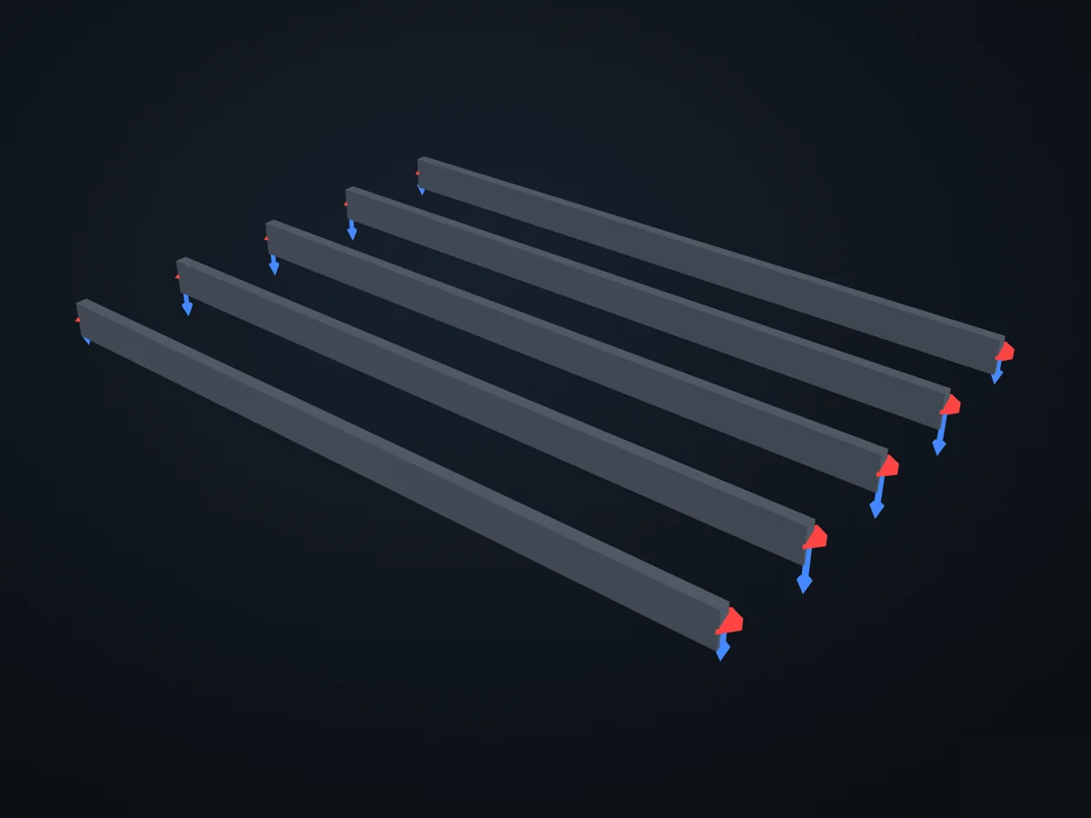
The model before it is solved: its parts, supports (red) and loads (blue).
Open in 3D turn it, cut it, hide parts: in xfea's viewer, in your browser
The script
Section titled “The script”examples/scripts/02_core_concepts/loads_and_bcs/tributary_area.py. Run it from the repository with uv run python examples/scripts/02_core_concepts/loads_and_bcs/tributary_area.py, or, with xfea-examples installed, xfea-examples run 02_core_concepts/loads_and_bcs/tributary_area.py.
from __future__ import annotations
import tempfilefrom pathlib import Path
from xfea.geometry import Polygon
from xfea.model import (    BeamElement,    ElasticIsotropic,    Model,    Node,    Part,    RectangularSection,)from xfea.problem import Problem, StaticStepfrom xfea.problem.tributary import compute_tributary_nodal_forces

# Geometry / materialL_X = 6_000.0        # [mm]  plate length in X (beam span)L_Y = 4_000.0        # [mm]  plate length in YN_BEAMS = 5          # beams at y = 0, 1000, 2000, 3000, 4000 mmSPACING_Y = L_Y / (N_BEAMS - 1)
PRESSURE = 5.0       # [N/mm²]  (= 5 MPa, heavy DL just to get big numbers)
MAX_PATCH_SIZE = 100.0   # [mm]  ~ 6000/60 patches along X, 4000/40 along Y

# Build the model: 5 parallel beams, 6 m long eachdef build_model():    steel = ElasticIsotropic(E=210_000.0, v=0.3, density=7.85e-9, name="S355")    sec = RectangularSection(w=100.0, h=300.0, material=steel, name="rect_100x300")
    model = Model(name="plate_on_ribs", description="Tributary-area demo")    part = Part(name="ribs")    model.add_part(part)
    beam_end_nodes: list[tuple[Node, Node]] = []    beams: list[BeamElement] = []    for k in range(N_BEAMS):        y = k * SPACING_Y        n1 = part.add_node(Node(xyz=[0.0, y, 0.0]))        n2 = part.add_node(Node(xyz=[L_X, y, 0.0]))        beams.append(            part.add_element(                BeamElement(                    nodes=[n1, n2], section=sec, orientation=[0.0, 1.0, 0.0]                )            )        )        beam_end_nodes.append((n1, n2))
    # BCs: pin the two ends of every beam (not needed for the    # load-distribution demo but keeps the model analysable).    all_ends = [n for ends in beam_end_nodes for n in ends]    model.add_pin_bc(nodes=all_ends)    model.assign_keys()
    return model, beams, beam_end_nodes

# Distribute + reportdef run():    model, beams, beam_end_nodes = build_model()
    plate = Polygon(        [            (0.0, 0.0, 0.0),            (L_X, 0.0, 0.0),            (L_X, L_Y, 0.0),            (0.0, L_Y, 0.0),        ]    )
    # --- The actual API ---    problem = model.add_problem(Problem(name="tributary_demo"))    step = problem.add_step(StaticStep(name="dead_load"))    step.add_tributary_area_load(        region=plate,        supports=beams,        pressure=PRESSURE,        direction=[0.0, 0.0, -1.0],        max_patch_size=MAX_PATCH_SIZE,        load_case="DL",    )
    # Also re-run the bare algorithm so we can visualise the patches.    nodal_forces, patches = compute_tributary_nodal_forces(        region=plate,        supports=beams,        pressure=PRESSURE,        direction=[0.0, 0.0, -1.0],        max_patch_size=MAX_PATCH_SIZE,    )
    # --- Console report ---    area = L_X * L_Y    expected_total = PRESSURE * area    print("=" * 72)    print("Plate on parallel ribs — tributary area demo")    print(f"  plate       : {L_X:.0f} × {L_Y:.0f} mm  = {area / 1e6:.2f} m²")    print(f"  ribs        : {N_BEAMS}, spacing {SPACING_Y:.0f} mm")    print(f"  pressure    : {PRESSURE:.2f} N/mm²  (× {area / 1e6:.2f} m² = "          f"{expected_total / 1e6:.2f} MN total)")    print(f"  max_patch_size : {MAX_PATCH_SIZE:.0f} mm  ({len(patches)} patches)")    print()    total_z = sum(f[2] for f in nodal_forces.values())    print(f"  Σ node forces (Z) : {total_z:+,.1f} N    "          f"(expected {-expected_total:+,.1f} N, "          f"error {abs(total_z + expected_total) / expected_total * 100:.4f} %)")    print()    print("  Per-beam load (Σ over the 2 end nodes):")    print("  ┌─────────┬─────────────┬───────────────┬──────────────┬──────────┐")    print("  │ beam    │   y  [mm]   │  FEA Σ Fz [N] │ analytical   │  err     │")    print("  ├─────────┼─────────────┼───────────────┼──────────────┼──────────┤")    for k, (n1, n2) in enumerate(beam_end_nodes):        trib_lo = 0.0 if k == 0 else (k - 0.5) * SPACING_Y        trib_hi = L_Y if k == N_BEAMS - 1 else (k + 0.5) * SPACING_Y        analyt_force_z = -PRESSURE * L_X * (trib_hi - trib_lo)        fea_force_z = (            nodal_forces.get(n1, [0, 0, 0])[2] + nodal_forces.get(n2, [0, 0, 0])[2]        )        err = (            abs(fea_force_z - analyt_force_z) / abs(analyt_force_z) * 100            if analyt_force_z            else 0.0        )        print(            f"  │ beam {k}  │  {k * SPACING_Y:>5.0f}      │ "            f"{fea_force_z:+13,.1f} │ {analyt_force_z:+12,.1f} │  {err:5.3f} % │"        )    print("  └─────────┴─────────────┴───────────────┴──────────────┴──────────┘")    print("=" * 72)    return plate, beams, beam_end_nodes, nodal_forces, patches

# Matplotlib visualisationdef plot(plate, beams, beam_end_nodes, nodal_forces, patches, out_png):    import matplotlib.pyplot as plt    from matplotlib.patches import Polygon as MplPolygon
    fig, ax = plt.subplots(figsize=(12, 8))
    # Plate outline (soft fill).    plate_pts = [(float(p.x), float(p.y)) for p in plate.points]    ax.add_patch(        MplPolygon(            plate_pts,            closed=True,            facecolor="lightyellow",            edgecolor="goldenrod",            linewidth=1.5,            alpha=0.6,            zorder=1,        )    )
    # Every triangular patch — assigned to its nearest beam, coloured    # by beam index so you can see the tributary polygons emerging.    from xfea.problem.tributary import _unpack_supports
    supports = _unpack_supports(beams)    cmap = plt.get_cmap("viridis", len(supports))    for p in patches:        c = p.centroid        best_d = float("inf")        best_i = 0        for i, s in enumerate(supports):            _, d, _ = s.nearest(c)            if d < best_d:                best_d = d                best_i = i        tri = MplPolygon(            [(p.a[0], p.a[1]), (p.b[0], p.b[1]), (p.c[0], p.c[1])],            closed=True,            facecolor=cmap(best_i),            edgecolor="none",            alpha=0.35,            zorder=2,        )        ax.add_patch(tri)
    # Beams.    max_beam_load = max(        abs(nodal_forces.get(n1, [0, 0, 0])[2] + nodal_forces.get(n2, [0, 0, 0])[2])        for n1, n2 in beam_end_nodes    )    for k, (n1, n2) in enumerate(beam_end_nodes):        fz_sum = abs(            nodal_forces.get(n1, [0, 0, 0])[2] + nodal_forces.get(n2, [0, 0, 0])[2]        )        lw = 2.0 + 6.0 * (fz_sum / max_beam_load if max_beam_load else 0.0)        ax.plot(            [float(n1.x), float(n2.x)],            [float(n1.y), float(n2.y)],            color="black",            linewidth=lw,            solid_capstyle="round",            zorder=4,        )        ax.annotate(            f"{fz_sum / 1e6:.1f} MN",            xy=(float(n1.x) - 120, float(n1.y)),            ha="right", va="center",            fontsize=8, color="black",        )
    # Node markers (force magnitude as marker size).    all_nodes = [n for pair in beam_end_nodes for n in pair]    xs = [float(n.x) for n in all_nodes]    ys = [float(n.y) for n in all_nodes]    fs = [abs(nodal_forces.get(n, [0, 0, 0])[2]) for n in all_nodes]    max_fs = max(fs) or 1.0    sizes = [40 + 200 * (f / max_fs) for f in fs]    ax.scatter(xs, ys, s=sizes, color="darkred", zorder=5, edgecolors="black")    for n, f in zip(all_nodes, fs):        ax.annotate(            f"{f / 1e6:.1f} MN",            xy=(float(n.x), float(n.y)),            xytext=(6, 6), textcoords="offset points",            fontsize=7, color="darkred", fontweight="semibold",        )
    ax.set_aspect("equal")    ax.set_xlabel("X (mm)")    ax.set_ylabel("Y (mm)")    ax.set_title(        f"Tributary area distribution — plate {L_X:.0f}×{L_Y:.0f} mm on {N_BEAMS} ribs\n"        f"p = {PRESSURE:.2f} N/mm², total = {PRESSURE * L_X * L_Y / 1e6:.1f} MN"    )    ax.grid(True, alpha=0.25, linestyle=":")    ax.margins(0.08)    fig.tight_layout()    fig.savefig(out_png, dpi=150)    print(f"\n  plot saved: {out_png}")    plt.show()

if __name__ == "__main__": plate, beams, beam_end_nodes, nodal_forces, patches = run() out_png = Path(tempfile.gettempdir()) / "xfea_tributary_demo.png" plot(plate, beams, beam_end_nodes, nodal_forces, patches, out_png)© 2026 Francesco Ranaudo · Text and pictures CC BY 4.0 · Code Elastic License 2.0 · how to reuse them