
Plane (2-D) heat-transfer analysis of a cross-section from a STEP file
Reads a planar STEP file describing one or more closed regions in the XY plane, at z = 0, where 2-D plane elements lie (without one, a 300 x 500 mm concrete beam section: x across it, y up it), meshes it with 2-D plane heat-transfer elements, applies an ISO 834 fire to a configurable subset of the boundary edges, and reports the 500 °C isotherm.
The mesh stays strictly 2-D — no extrusion, no through-thickness gradient. That makes this the right tool when you only care about the in-plane temperature field of a long prismatic cross-section (slab, wall, beam web, hollow section, …) and don’t want to pay for a 3-D solid model.
# default: a 300 x 500 mm beam section (or the file at DEFAULT_STEP_PATH); fire on the bottom edgepython thermal_2d_cross_section_step.py
# custom geometrypython thermal_2d_cross_section_step.py path/to/section.stp
# change which edges are fire-exposed via FIRE_SIDE below# ("ymin" / "ymax" / "xmin" / "xmax" / "any")
Inputs the user is expected to swap in
Section titled “Inputs the user is expected to swap in”DEFAULT_STEP_PATH(or the first argument) — your planar STEP. Multiple disjoint loops in the same file are fine: Gmsh imports each region as its own OCC face and the mesher meshes them all into a singlePart(separate regions remain numerically disconnected unless they share nodes).FIRE_SIDE— which side of the bounding box receives the fire. For more complex selectors edit_edge_on_sidedirectly.- Mesh sizes (
MESH_MIN/MESH_MAX), fire duration, material curves, initial temperature — all near the top.
Disjointed regions
Section titled “Disjointed regions”If your STEP carries N disconnected regions and you want different
materials / sections per region, build N parts and assign
part.base_geometry to a STEP that only contains that region (split
the file upstream, or use OCC to extract one face at a time). Putting
everything in one part with one section is the simplest start — copy
this script and split later if needed.
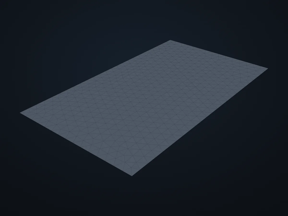
The model before it is solved: its parts, supports (red) and loads (blue).
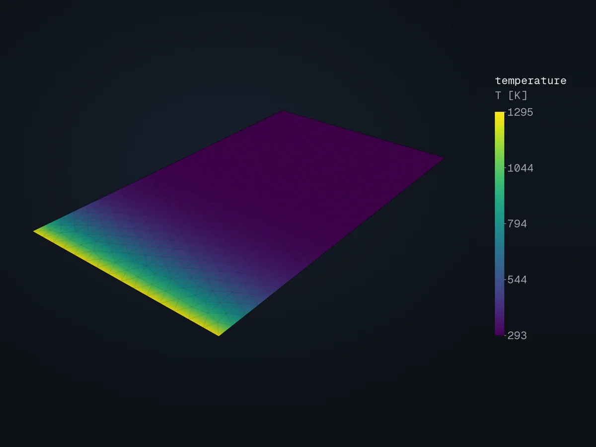
The model, coloured by temperature (T [K]), in xfea’s 3D viewer.
Open in 3D turn it, cut it, pick any field: in xfea's viewer, in your browser
The script
Section titled “The script”examples/scripts/02_core_concepts/thermal_analysis/thermal_2d_cross_section_step.py. Run it from the repository with uv run python examples/scripts/02_core_concepts/thermal_analysis/thermal_2d_cross_section_step.py, or, with xfea-examples installed, xfea-examples run 02_core_concepts/thermal_analysis/thermal_2d_cross_section_step.py.
from __future__ import annotations
import argparseimport osimport sys
import matplotlib.pyplot as pltimport matplotlib.tri as mtriimport numpy as np
from xfea.meshing import MeshingSettingsfrom xfea.model import (    BoundaryInterface,    Convection,    Model,    Part,    PlaneHeatTransferSection,    Radiation,    ThermalElasticIsotropic,)from xfea.problem import HeatTransferStep, Problemfrom xfea.results import TemperatureFieldResults
from xfea_examples import out_dirfrom xfea_tools import iso834from xfea.geometry import Mesh

# Configuration — edit theseDEFAULT_STEP_PATH = ""        # your planar STEP; empty: the beam section belowBEAM_WIDTH, BEAM_DEPTH = 300.0, 500.0                    # [mm] the section used without a STEP fileFIRE_SIDE = "ymin"                                       # "xmin"|"xmax"|"ymin"|"ymax"|"any"
FIRE_DURATION = 7200          # [s]   ISO 834 exposure (R120)T_INITIAL = 293.15            # [K]   20 °C ambientT_ISOTHERM_K = 773.15         # [K]   500 °C isotherm to extract
MESH_MIN = 5                  # [mm]MESH_MAX = 20                 # [mm]
# EN 1991-1-2 §3.1 — generic fire-exposed boundary propertiesH_CONV = 25.0e-3              # [mW/(mm^2·K)]   = 25 W/(m^2·K)EPS_RAD = 0.7                 # [-]
# Concrete with EN 1992-1-2 §3.3 temperature-dependent thermal properties.# Swap the helpers below to model a different material (steel: EN 1993-1-2,# timber: EN 1995-1-2, etc.) — keep the (value, T_kelvin) tuple format.DENSITY = 2.3e-9              # [t/mm^3] = 2300 kg/m^3E_DUMMY = 30_000              # [MPa] unused in pure HT but the material expects itNU_DUMMY = 0.2

def _ec2_conductivity(T_celsius: float) -> float:    """EN 1992-1-2 §3.3.1 — siliceous concrete, lower limit."""    T100 = T_celsius / 100.0    return max(1.36 - 0.136 * T100 + 0.0057 * T100**2, 0.5)

def _ec2_specific_heat(T_celsius: float) -> float:    """EN 1992-1-2 §3.3.2 — siliceous concrete, u = 1.5 % moisture peak."""    if T_celsius <= 100:        return 900.0    if T_celsius <= 115:        return 900.0 + (1470.0 - 900.0) * (T_celsius - 100) / 15.0    if T_celsius <= 200:        return 1470.0 + (1000.0 - 1470.0) * (T_celsius - 115) / 85.0    if T_celsius <= 400:        return 1000.0 + (T_celsius - 200) / 2.0    return 1100.0

# CLIparser = argparse.ArgumentParser(description=__doc__.splitlines()[0])parser.add_argument(    "step", nargs="?", default=DEFAULT_STEP_PATH,    help="Planar STEP file (defaults to DEFAULT_STEP_PATH).",)parser.add_argument(    "--fire-side", default=FIRE_SIDE,    choices=["xmin", "xmax", "ymin", "ymax", "any"],    help="Which side of the bbox is fire-exposed. 'any' = whole perimeter.",)parser.add_argument("--duration", type=float, default=FIRE_DURATION,                    help="Exposure time in seconds.")args = parser.parse_args()
if args.step and not os.path.isfile(args.step):    sys.exit(        f"STEP file not found: {args.step}\n"        "Pass the path as an argument or edit DEFAULT_STEP_PATH at the top."    )if args.step:    geometry = args.stepelse:  # a rectangular beam section in the XY plane, soffit at y = 0    geometry = Mesh.from_vertices_and_faces(        [(-BEAM_WIDTH / 2, 0.0, 0.0), (BEAM_WIDTH / 2, 0.0, 0.0),         (BEAM_WIDTH / 2, BEAM_DEPTH, 0.0), (-BEAM_WIDTH / 2, BEAM_DEPTH, 0.0)],        [[0, 1, 2, 3]],    )
OUTPUT_DIR = out_dir("thermal_2d_cross_section_step")print(f"Geometry      : {args.step or f'beam section {BEAM_WIDTH:.0f} x {BEAM_DEPTH:.0f} mm'}")print(f"Fire side     : {args.fire_side}")print(f"Duration      : {args.duration:.0f} s  (R{int(args.duration / 60)})")print(f"Output dir    : {OUTPUT_DIR}")

# Stage 1 — material, section, meshprint("\n" + "=" * 60)print("Stage 1: Material + Section + 2-D Mesh")print("=" * 60)
# Sample densely between 100 and 200 °C so the moisture peak at 115 °C is# resolved by the piecewise-linear table that the solver interpolates from._temps_C = sorted(set(    list(range(20, 101, 20))    + list(range(100, 201, 5))    + list(range(200, 1201, 50))))k_table = [(_ec2_conductivity(T), T + 273.15) for T in _temps_C]# SI-mm: c [mJ/(t·K)] = c [J/(kg·K)] × 1e6c_table = [(_ec2_specific_heat(T) * 1e6, T + 273.15) for T in _temps_C]
material = ThermalElasticIsotropic(    k=k_table, c=c_table,    E=E_DUMMY, v=NU_DUMMY, density=DENSITY,)# Out-of-plane thickness ``t`` is purely a flux-integral factor — keep# at 1 mm unless you want to compare totals against a 3-D run.section = PlaneHeatTransferSection(material=material, t=1.0)
model = Model(name="thermal_2d_cross_section_step")part = model.add_part(Part(name="section"))part.base_geometry = geometrypart.mesh(settings=MeshingSettings(min=MESH_MIN, max=MESH_MAX), section=section)print(f"  Mesh: {len(list(part.nodes))} nodes, {len(list(part.elements))} elements")

# Stage 2 — boundary conditionsprint("\n" + "=" * 60)print("Stage 2: Boundary conditions (ISO 834 fire)")print("=" * 60)
# Build the bbox manually rather than calling ``on_bbox`` because that# helper is wired for faces, not edges. The logic is identical: "the# edge lies on the chosen bbox side if all its node coords sit on the# corresponding plane within tol".nodes = list(part.nodes)x_min = min(float(n.x) for n in nodes)x_max = max(float(n.x) for n in nodes)y_min = min(float(n.y) for n in nodes)y_max = max(float(n.y) for n in nodes)bbox = {"xmin": ("x", x_min), "xmax": ("x", x_max),        "ymin": ("y", y_min), "ymax": ("y", y_max)}TOL = 1e-3 * max(x_max - x_min, y_max - y_min)

def _edge_on_side(edge, side: str) -> bool:    if side == "any":        return True    axis, target = bbox[side]    return all(abs(getattr(n, axis) - target) < TOL for n in edge.nodes)

boundary_edges = part.find_boundary_edges()fire_edges = boundary_edges.subgroup(lambda e: _edge_on_side(e, args.fire_side))fire_group = part.add_group(fire_edges)fire_group.name = "fire_exposed_edges"print(f"  Boundary edges          : {len(list(boundary_edges))}")print(f"  Fire-exposed (on {args.fire_side:>4}) : {len(list(fire_edges))}")if len(list(fire_edges)) == 0:    sys.exit(        f"No boundary edges lie on side {args.fire_side!r}. "        "Inspect the geometry or pick a different --fire-side."    )
fire_curve = iso834(int(args.duration), dt=60, name="ISO834")convection = Convection(    h=H_CONV,    temperature_value=1.0,    temperature_amplitude=fire_curve,)radiation = Radiation(    eps=EPS_RAD,    temperature_value=1.0,    temperature_amplitude=fire_curve,)model.add_interface(BoundaryInterface(master=fire_group, behavior=convection))model.add_interface(BoundaryInterface(master=fire_group, behavior=radiation))model.add_uniform_thermal_ics_field(T0=T_INITIAL, nodes=part.nodes)

# Stage 3 — transient heat transferprint("\n" + "=" * 60)print(f"Stage 3: Transient heat transfer (R{int(args.duration / 60)})")print("=" * 60)
problem = model.add_problem(Problem(name="fire"))step = problem.add_step(HeatTransferStep(    name="fire_exposure",    time=args.duration,    initial_inc_size=2,    min_inc_size=0.1,    max_inc_size=60,    max_increments=10_000,    max_temp_delta=50,    steady_state=False,))temp = TemperatureFieldResults()step.add_field_outputs([temp])
print("  Running the solver...")problem.analyse_and_extract(path=OUTPUT_DIR, verbose=True)
t_final_min = temp.get_min_result("T", time=args.duration)t_final_max = temp.get_max_result("T", time=args.duration)print(    f"  Final temperatures:  min = {float(t_final_min.T) - 273.15:.1f} °C, "    f"max = {float(t_final_max.T) - 273.15:.1f} °C")

# Stage 4 — 500 °C isotherm plotprint("\n" + "=" * 60)print("Stage 4: 500 °C isotherm")print("=" * 60)
results = temp.get_results(time=args.duration)xs = np.array([r.location._x for r in results])ys = np.array([r.location._y for r in results])ts = np.array([float(r.T) - 273.15 for r in results])
# The Triangulation defaults to a Delaunay over (x,y) which can bridge# concave regions or holes. For a quick visual that's usually fine; for# strict masking, switch to per-element triangle indices via ``part.elements``.triang = mtri.Triangulation(xs, ys)
fig, ax = plt.subplots(figsize=(10, 8))filled = ax.tricontourf(triang, ts, levels=32, cmap="hot_r")fig.colorbar(filled, ax=ax, label="Temperature [°C]")contour = ax.tricontour(triang, ts, levels=[500.0], colors="cyan", linewidths=2)
# Optional: EN 1992-1-2 insulation criterion ΔT ≤ 140 KT_LIMIT_C = 140.0T_INSULATION_C = (T_INITIAL + T_LIMIT_C) - 273.15ax.tricontour(triang, ts, levels=[T_INSULATION_C], colors="darkgreen", linewidths=1.5)
ax.set_xlabel("x [mm]")ax.set_ylabel("y [mm]")ax.set_aspect("equal")ax.set_title(    f"2-D cross-section — ISO 834 R{int(args.duration / 60)} on {args.fire_side}\n"    f"500 °C isotherm (cyan), T ≤ T₀ + 140 K (dark green)")ax.grid(True, alpha=0.3)fig.tight_layout()
plot_path = os.path.join(OUTPUT_DIR, f"thermal_field_R{int(args.duration / 60)}.png")fig.savefig(plot_path, dpi=150)plt.close(fig)print(f"  Plot saved: {plot_path}")
# Dump the 500 °C polyline so you can overlay it on structural drawings.poly_path = os.path.join(OUTPUT_DIR, "isotherm_500_polyline.txt")with open(poly_path, "w") as fh:    fh.write(f"# 500 C isotherm after R{int(args.duration / 60)} ISO 834\n")    fh.write("# x[mm]  y[mm]   (blank line separates disconnected segments)\n")    n_seg = n_vert = 0    for path in contour.get_paths():        verts = path.vertices        if len(verts) == 0:            continue        n_seg += 1        for x, y in verts:            fh.write(f"{x:10.3f} {y:10.3f}\n")            n_vert += 1        fh.write("\n")print(f"  Polyline saved: {poly_path}  ({n_seg} segments, {n_vert} vertices)")
print("\nDone.")© 2026 Francesco Ranaudo · Text and pictures CC BY 4.0 · Code Elastic License 2.0 · how to reuse them